New gene page, new Bgee interface

Yesterday we have released a major update of our web interface:

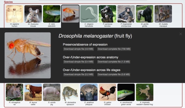
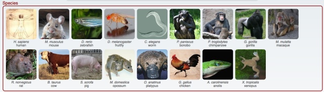
The download functionality remains the same, as does the data (processing for the next release is just starting with the new Ensembl release – we love Ensembl). It’s just easier to find and use (we hope! Feedback welcome at bgee@sib.swiss).

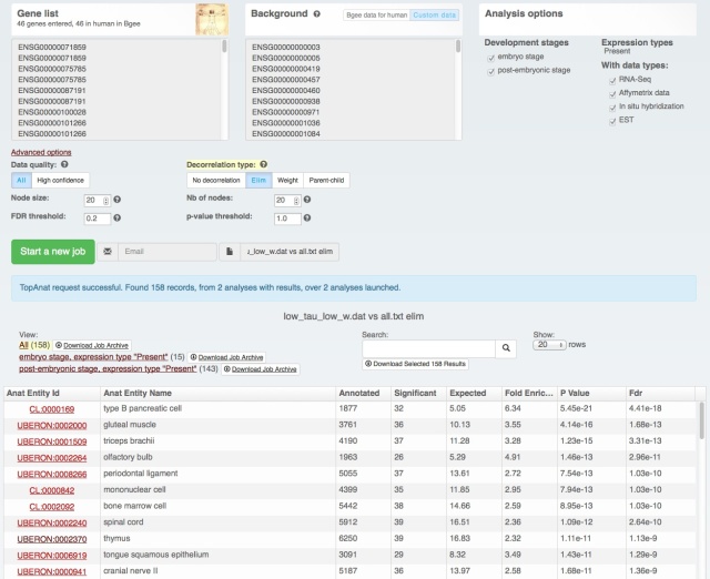
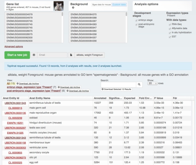
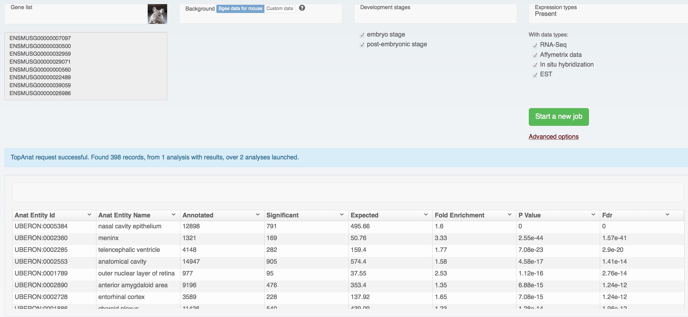
We also rolled out some improvements in TopAnat:

• clearer access to documentation;
• clearer access to example datasets;
• correction of a bug in column sorting.

But the major functional improvement is the new gene page (click on the picture, or on “Gene search” on the Bgee homepage):

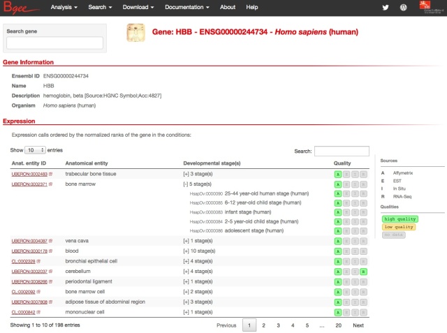
All expression information for each gene is summarized. It may look easy, but it took us quite a bit of thinking, and programming, and re-thinking, and re-programming, to find a presentation which satisfied us.

The problem is that we have really a lot of information on expression patterns for each gene, especially in major model species. Hemoglobin beta of human, presented above, is expressed in 696 combinations anatomical structure – life stage; 8108 with full propagation in the anatomical ontology. And for each of these, we may have several evidence lines, from different types of expression data. Yet we know that for this gene the most important expression is in blood cells, thus bone marrow, blood or heart should come on top. Showing the amount of data from the download files:

> grep ENSG00000244734 Homo_sapiens_expr-simple.tsv | wc
696 9249 83866
> grep ENSG00000244734 Homo_sapiens_expr-complete.tsv | wc
8108 266136 1678370

The challenge is to summarize this without hiding too much of the relevant information, but while putting the most important information forward clearly. For this, we made the following choices:

• anatomical structures are put forward by default; life stages (development and aging) are available by unfolding for each anatomical structure (as illustrated above with bone marrow).
• for each anatomical structure, we compute a normalized rank. This is rather complicated, as we need to weight for the fact that RNA-seq typically covers all genes, and in situ hybridization only a few, with microarrays and ESTs in between. We start by ranking genes inside each experiment.  Briefly, the maximum rank is used as a normalizing factor. Maximum rank takes into account the number of genes called, but also how well they are differentiated: if 100 genes are called by in situ hybridization in a condition, but 99 have 1 evidence each and 1 gene has 10 evidence lines, the max rank is lower than if 100 genes each have different numbers of ESTs. For Affymetrix there is a normalization between experiments for a same condition. For in situ hybridization, all evidence for a given condition is put together as one “pseudo-experiment”, and the number of lines of evidence for a gene is used for ranking. Then each gene gets a mean rank per data type and per condition, and these are normalized. And these are then averaged for a condition, weighting again by max ranks. We forgive you if you didn’t completely follow. The important things are: do the most relevant conditions come on top? (They seem to.) Is the data behind it available? (Yes, see the download pages.)
• call quality is not taken into account, as we did not find that it added anything to the ranking; this might lead us to reconsider our evaluation of call quality in the future, but that’s another story.
• expression data is presented simply in the form of little vignettes indicating that a type of data was used to call a condition.

This is the first version of this gene page, and obviously more will need to be added to it, such as links to the data, homology links, links to other databases, and more elaborate search features.

More details on the algorithm and comparisons to other databases on Marc’s blog.

But we are already very proud of how well the ranking algorithm works. It was tested on several genes, such as hemoglobin, and we consistently get the most biologically relevant structures on top. Importantly, this is done without sacrificing specificity: we do not necessarily push to the top simply the more general anatomical terms, such as “vascular system”. And while the weighting scheme down weights in situ data when it is scarce and thus uninformative, good in situ data can push anatomical structures to the top of this list, as in the example of zebrafish insulin expression in the pancreas.

Confirming that autism and epilepsy genes are expressed in specific brain areas

Recently we presented on this blog a quick-and-dirty analysis of genes with the keyword “autism” from the GWAS Catalog at EBI. But recently, Jabbari and Nürnberg have published a more thorough study of autism and epilepsy candidate genes:

Jabbari and Nürnberg 2016 A genomic view on epilepsy and autism candidate genes Genomics doi:10.1016/j.ygeno.2016.01.001

The supplementary data of this paper provides a list of candidate genes from ClinVar, exome sequencing, and a gene panel from Lemke et al.

Analyzing all their genes in TopAnat, we get clear enrichment for specific brain substructures (as always, click on images to go to original results):

In Jabbari and Nürnberg they discuss differences in GO enrichment between the Lemke genes and the exome+ClinVar. What of anatomical structure enrichment?

Here is the enrichment with exome+ClinVar only:

And here it is with the gene panel only:

Seven of the top 20 are in common: nucleus accumbens, hypothalamus, superior frontal gyrus, dorsolateral prefrontal cortex, caudate nucleus, putamen and spinal cord. And most others are found lower ranked. Overall, less than 20% of the anatomical terms found with ClinVar + exome are not found with the gene panel, at an FDR of 20%. Thus, the two approaches yield extremely similar gene lists in terms of their expression patterns. Which is reassuring.

Gene expression enrichment tests are sensitive enough to detect where your background data came from #TopAnat

When you invent such a cool toy as TopAnat, you play with it. And then sometimes, you’re afraid that you might have broken it. But then, maybe it’s more robust than you expected. This is such a story.

One lab member was analyzing a large RNA-seq data set, with 27 human tissues (from Fagerberg et al. 2014). Another lab member decided to have a look at the ubiquitously expressed genes from this set which have conserved protein sequences (low dN/dS). Using TopAnat, the person found very significant tissue enrichments (click on picture to see analysis):

This was very surprising, since the data were selected to not be tissue-specific. A bug was suspected. The result was robust to changes in decorrelation algorithm, and after verification, yes TopAnat does remove redundancy in the input gene list.

A potential biological explanation was that tissue-specific genes may be more in common in some tissues, which would create an apparent enrichment for ubiquitous genes in the other tissues. But then we did a simple control: a random set of the genes called expressed in any of the 27 tissues (i.e., the genes on which tissue specificity could be calculated):

Ooo-Kay. Again very significant, and similar anatomical entities. But these are random genes, right? Well, randomly from expression over 27 tissues. Which surely means mostly random? Ah-ha. What are these tissues?

colon, kidney, liver, pancreas, lung, prostate, brain, stomach, spleen, lymphnode, appendix, small intestine, adrenal gland, duodenum, fat, endometrium, placenta, testis, gallbladder, urinary bladder, thyroid, esophagus, heart, skin, ovary, bone marry, salivary gland

Suddenly the results above start to make sense. And indeed, if we now take randomly from the full list of genes used for the RNA-seq mapping, not restricting to those called present at least once, we get:

Nothing significant!

We were detecting the signal of which specific tissues were sampled in this large dataset of 27 human tissues. A presumably subtle signal, but which left enough trace in the data that we could detect it. This shows both the sensitivity of the TopAnat test, and the power which comes from integrating so much data of different types into Bgee and TopAnat. Our toy was not broken, it was showing off what a cool toy it really is.

We hope that this convinces you that all data is biased TopAnat can detect relevant signal. 🙂

Update: here is the missing test from this story: the original low dN/dS ubiquitously expressed gene list, with the background set to genes called present at least once in Fagerberg et al 2014 (removing the sampling bias):

When fold-enrichment is more informative than p-values: #TopAnat analysis of autism genes from GWAS

In a recent post on this blog we saw how to analyze results from a breast cancer GWAS. In that case, we did not have very strong expectations of tissue-specificity for the genes; it was more of an exploratory analysis.

This time, let’s do the same but searching GWAS Catalog for the term “autism”. Here we have a clear expectation of finding genes expressed in the brain.

Using the same methodology as for breast cancer, we find 87 genes with a significant SNP inside the gene, and we obtain the following in TopAnat:

We notice that the top terms, ranked by FDR (the default), are not necessarily brain related. Other the other hand, looking down the list we notice some higher fold-changes. Ranking by “Fold enrichment” (just click on the head of column), we get:

Now all the top terms are parts of the brain! In case you are wondering what the paraflocculus is, you can click on the Uberon ID and get to the definition: it’s a cerebellar
tonsil.

What this illustrates, and is well known in other contexts, is that the p-value (and its close friend the FDR) only takes you so far, since it is so dependent on sample size. The top terms by FDR have very large numbers of genes called expressed in them (≈20k!), whereas the more specific brain parts have a few thousand “only” genes expressed.

Thus we have a strong biological signal in the patterns of gene expression, but we have to be weary of relying on p-values. As always in statistics. 😉

 

Update: see also this more recent post on autism and epilepsy genes.

#TopAnat where are genes significant in a breast cancer GWAS expressed?

Genome Wide Association Studies (GWAS) report many significant SNPs, which may be associated to many genes. How can we make sense of them? One way is to compute enrichment of the resulting gene list for properties of interest.

For example expression patterns! Thanks to TopAnat.

Let’s try this with breast cancer associated genes. First, we download the complete file of the GWAS catalog at EBI (awesome tool!). Then let’s do some simple “nosql” parsing:

grep "breast cancer" gwas_catalog_v1.0.1-downloaded_2016-01-08.tsv | cut -f18

This gives us the genes which have a breast cancer associated SNP within the gene. It gives us Entrez IDs, and TopAnat beta only takes Ensembl IDs (I am told that GWAS catalog will soon have Ensembl, and we are pushing to support other identifiers in TopAnat…). So let’s send this list to biomart:

• chose Ensembl genes
• chose Homo sapiens genes
• in Filters, chose Gene, “Input external references ID list”, and use our list of Entrez IDs
• in Attributes, remove Transcript ID
• in Results, we will get the list of Ensembl gene IDs.

Similarly, we can recover the genes which have significant SNPs upstream or downstream of the gene:

grep "breast cancer" gwas_catalog_v1.0.1-downloaded_2016-01-08.tsv | cut -f16,17

Now, let’s paste our lists of Ensembl gene IDs into TopAnat.

We chose the following options:

• background: all Bgee data, because we expect all genes to be detectable in GWAS; it is true that there might be a bias for gene length (longer genes have more SNPs by chance), which we will try to control for.
• decorrelation type: Weight, which allows to reduce the redundancy of the results by down-weighting less specific anatomical terms (organs, systems) relative to more specific ones (cell types, tissues).

We get 140 anatomical structures with FDR<0.2, which shows that there is some signal. It is clear that the top hits by p-value are enriched in the female reproductive system, and for epithelial tissues. Ranking them by fold-change, we obtain lacrimal gland on top, with a 3 fold enrichment relative to chance (p = 6.10E-07).

Of note, the same gene list put into the gene ontology enrichment tool at GOrilla gives many “positive regulation” terms, as well as weaker signal for prostate and muscle-related terms. Prostate is significant in the TopAnat analysis (p = 3.96e-21), as are 5 muscle types.

Let’s now look at the genes which are neighboring non genic SNPs:

First, the signal is weaker, but less good p-values and slightly less anatomical terms. Second, we get again epithelial tissues on top, but not so much reproductive system (although vagina is significant with an enrichment of 1.66 and p = 2.52e-9). Third, lacrimal gland is again the top enriched term (enrichment of 2.69, p = 0.00408).

The writer of this post is not a specialist of breast cancer, but a rapid search tells us that:

Of all metastatic tumors to the orbit, breast carcinoma is considered to be the most prevalent primary tumor, accounting for 29% to 70% of all metastases.

(source)

Finally, as a simple control for gene length, here is the TopAnat result for the 500 longest human genes (according to Ensembl):

Lacrimal gland comes out, although weakly (enrichment 1.53, p = 0.0205), as does prostate. There are some components of the reproductive and mammary systems, such as “subdivision of uterine tube”, “epithelium of mammary gland”, “mammalian vulva” or “mammary gland”. (Hey, neat trick: you can filter terms by using the “Search” box above the table.)

Of course, more analyses would be needed to get to solid conclusions. This illustrates how TopAnat can provide additional biological information on gene lists from large scale scans.

The contribution of #RNAseq, #microarrays, in situ hybridization and ESTs to #TopAnat gene enrichment signal

In Bgee, we integrate gene expression data from RNA-seq, Affymetrix microarrays, ESTs and in situ hybridization data. It is natural to think that with RNA-seq being so powerful, we should not bother with other sources of information.

Yet we still have an order much more data with microarrays: in Bgee release 13, we have in total:

• 41 RNA-seq experiments, for 526 libraries.
• 1170 microarray experiments, for 13070 chips.

In situ hybridization provides an amazing level of anatomical detail which is way beyond what other techniques can offer for now. And ESTs? Well let’s check.

In TopAnat, we can compute enrichment of gene lists for expression in anatomical structures (organs, tissues, cell types) based on the integration of all data, or only some subtypes:

So let’s try. Starting the example provided in “Quickstart” of “mouse genes annotated to GO term “spermatogenesis”. We expect these genes to be very tissue-specific (see also our recent analysis in Briefings in Bioinformatics), so it should be an easy case for each data type. We will choose one datatype at a time. To give each datatype its chance, we will perform these analyses with the lowest stringency: “Data quality” to “All”, no Decorrelation algorithm, and removing the FDR≤0.2 limit for reporting results.

Here are the results (click on images to go to the results on the TopAnat webpage):

With RNA-seq we obtain relevant organs, but very few. Essentially all the signal comes from testis, which is part of the male reproductive system, gonad, etc. The signal that we do get is very significant, which is reassuring.

With microarrays, we have more tissues and organs significant, with some more detailed structures. This is probably because we have many more experiments from microarrays, and thus some more detailed, than for RNA-seq. Again, statistics are good, and the organs reported are relevant. Don’t throw those microarray data quite yet! (Keep in mind though that Bgee only uses curated microarrays which are from healthy wild type and pass quality control.) On the other hand, notice that from our 457 genes, 442 were called expressed in gonad with RNA-seq, but only 402 with microarray: it is probable that lowly expressed genes were missed by the microarray experiments.

In situ hybridization gives us much more detailed structures, with very good statistical significance. Because we didn’t use any decorrelation, the results are difficult to read: a germ cell is a eukaryotic cell, and we get this information although it is not of great interest.

That’s a point in favor of using decorrelation for most analyses. For example, if we redo that analysis with “Weight”, which removes most of the signal due to the non independence of these structures (spermatocyte is a male germ cell, which is a cell, etc), we obtain: the following structures (FDR <0.2):

male germ cell; male reproductive organ; ooblast; hindgut diverticulum (mouse); gonad; testis sex cord; pharyngeal arch 2; membranous layer; meiotic oocytes (mouse); ventricular zone; entire extraembryonic component; otic pit; 1st arch maxillary component.

We see here the great level of detail obtained with in situ hybridizations. On the other hand, for each structure we have 13-28 genes only called present.

Finally, for ESTs we obtain something similar to RNA-seq, although with less genes called present. It is noteworthy that there is so much biological signal in ESTs, although this type of data is nowadays largely neglected.

To wrap up this comparison, first the table of all structures called by at least one data type alone, FDR<0.2, using the Weight algorithm (links to the analyses: RNA-seq, microarrays, in situ, ESTs):

data type	anatEntityName	significant	foldEnrichment	pValue	FDR
RNAseq	testis	433	1.259	2.16E-30	4.08E-28
microarray	seminiferous tubule of testis	351	1.411	7.91E-30	7.37E-27
insitu	male germ cell	17	7.556	2.88E-11	2.15E-08
insitu	male reproductive organ	19	3.506	3.01E-08	0.0000112
insitu	ooblast	9	7.965	0.00000142	0.00267
insitu	hindgut diverticulum (mouse)	10	5.495	0.0000122	0.01073
insitu	gonad	114	1.555	0.0000171	0.01073
insitu	testis sex cord	21	2.668	0.0000407	0.01914
insitu	pharyngeal arch 2	23	2.312	0.000237	0.08915
insitu	membranous layer	21	2.253	0.000431	0.13511
insitu	meiotic oocytes (mouse)	8	4.324	0.000433	0.108
insitu	ventricular zone	28	1.931	0.000623	0.16758
insitu	entire extraembryonic component	34	2.457	0.000738	0.17353
insitu	otic pit	10	3.311	0.000888	0.18575
insitu	1st arch maxillary component	21	2.111	0.00102	0.19113
EST	male reproductive system	312	1.495	1.36E-35	6.70E-33

Second, the analysis with Weight algorithm, FDR<0.2, all data integrated:

Note how the integration of data types allows us to obtain both statistical power and anatomical specificity.

 

Take-home messages:

• if you have good quality older data, don’t throw it, it contains good biology;
• when you use TopAnat, integrate all data and use decorrelation.

What makes #TopAnat special relative to classical #GeneOntology enrichment?

In bioinformatics and genomics, we are all familiar with GO (Gene Ontology) enrichment test. You take a gene list, paste it into a tool such as Gorilla, PANTHER, or others, and obtain a list of terms which are enriched in your gene list.

How this works is that each gene in your gene list has GO terms associated to it, through experimental or computational evidence. For each term, we can thus count how many times it is associated to a gene in your list, and compare this to the count which is expected from a random gene list of the same size (same number of genes).

TopAnat does the same (see also here), but each gene has anatomical terms associated to it. And here is an important difference: all associations are experimental. TopAnat uses Bgee expression calls, which are from an integration in situ hybridizations, RNA-seq, microarrays, and ESTs. No gene is associated to “brain” because its ortholog is, or because it is paralogous to another gene expressed in the brain, or shares a domain which is frequently found in brain genes. A gene is only associated to the brain because we have experimental evidence that it is expressed in the brain or a sub-structure of the brain (e.g., all genes expressed in cerebellum are expressed in brain).

Because we have so much expression data (also see this talk), and it is increasing, we actually do have such annotations for most genes. Because RNA-seq is applicable to all species, we have such annotations for all species in Bgee (17 at present). Because in situ hybridizations are very precise, we have such annotations for many tissues and cell types in non model (or emerging model) organisms, from cow to platypus and anole lizard.

This is particularly interesting because expression patterns closely match the type of function covered by the Biological Process of the GO, which is the hardest to predict (e.g., CAFA). Here, we do not predict, we report.

Finally, because Bgee only includes manually curated data from healthy wild-type samples, the associations correspond only to the “normal” function of the genes. This is not to say that the implication of genes in diseases or genetic modifications are not interesting, but they should not be confused with the normal function.

When TopAnat provides you a list of anatomical terms, you can know that:

• they are experimentally supported in the species which you are studying;
• they integrate all available information, not only one datatype;
• they only represent healthy wild-type gene functions.

Enjoy TopAnat!

#TopAnat: GO-like enrichment of anatomical terms mapped to genes by expression patterns

Update: This was the first blogpost on TopAnat. There are now quite a few more, under the tag TopAnat.

We are glad to roll out the first public beta version of our new tool, TopAnat:

http://bgee.org/?page=top_anat

TopAnat uses the classical GO-enrichment approach (specifically, from TopGO), comparing terms associated to your gene list to those associated to a background list, and reports terms which are over-represented. The main differences with GO-enrichment are that

1. the ontology used described anatomy rather than gene function;
2. the association between genes and ontology terms is obtained from gene expression patterns rather than annotation.

Like for GO-enrichment, you can use a default background of all genes in your organism with expression data in Bgee, or you can upload your own background set. Because this is based on TopGO, you can use several algorithms to decorrelate the ontology, to avoid reporting terms which are annotated to the same genes because of part_of relations, such as “prefrontal cortex” and “frontal cortex”. The options are:

• No decorrelation
• Elim (by default)
• Weigth (update: now by default)
• Parent-child.

For now, genes are only associated to anatomical structures through present / absent calls, i.e. you will obtain structures with more “present” calls than expected by chance. In the future, we will be adding enrichment based on expression being higher in some tissues than others (“over-expression”). The test as it is shows that present calls of expression already contain a lot of biologically relevant information. For example, here are the top anatomical structures for genes associated to the GO term “neurological system process” in mouse (see full results here; loading can be a bit slow):

Because developmental expression patterns can be very different from adult ones, we compute enrichment twice by default, for expression patterns in development (“embryo stage”) and in new born to adult (“post embryonic stage”). If you feel that more detailed breakdown is needed, please ask us, although note that in some cases we will probably lack statistical power.

Because Bgee annotates only healthy wild type expression data, you can rest assured that the results are not pulled by expression in tumors, KOs, or other diseases, but are representative of healthy biological processes.

And because Bgee integrates in situ hybridization with microarrays and RNA-seq, you can obtain very detailed anatomical information in mouse, fly, zebrafish or nematode, as shown in the mouse neurological process genes above.

Finally, because Bgee annotates expression data from  17 species, you can immediately perform tests in all these species. Although be warned that in species with less data tests will lack power. Example : tissue enrichment of genes on the X chromosomes of platypus (loading can be a bit slow). Note that while the FDR is not significant (lack of power), the top structures make sense for sex chromosomes.

We will be testing and improving TopAnat over the next weeks, and we already look forward to playing with it. We are confident that it will be useful, and hope that many of you will be able to use it to gain biological insight into those gene lists you get in this big data biology age.

TopAnat is based on an adaptation by Julien Roux of TopGO, by Adrian Alexa. It has been incorporated into Bgee by the Bgee team (names tagged Bgee in this list), and the graphical user interface has been developped by the SIB WebTeam. All data in Bgee are annotated to the Uberon ontology.

10 million calls of differential gene expression for 11 species, from #RNAseq and #microarray

Continuing to roll out Bgee release 13 (see first installment), we now provide pre-computed files of differential gene expression. As for present / absent calls, files are organized per species, and come in “simple” and “complete” versions.

A test of differential expression is made when one experiment has several conditions, with replicates for each condition. We separate comparisons of different tissues in the same developmental stage (“anatomy”) from comparisons of the same tissue at different life history stages (“development” – this includes aging). For each gene and condition, a gene can be called “over-expressed”, if it is more expressed than in the average of conditions, “under-expressed”, if it is less expressed than in the average of conditions, or “no diff expression” otherwise. The test is a modified ANOVA.

A same gene in a same condition can be called from several experiments. These may use the same or different platforms (RNA-seq or microarray), and compare the same or different conditions (different combinations of tissue and stage). For a given technique, we resolve conflicts (e.g., the same gene called over- and under-expressed in liver in different experiments) based on a voting system weighted by p-values. Importantly, whenever this is a conflict, the summary call that we provide is noted “low quality”.High quality calls are those with no conflict and p<0.01. We provide summary calls from different experimental types separately in the “complete” file, while we provide one overall summary call per gene-condition combination in the “simple” file. In the latter case, conflicts between different techniques a summarized by an “ambiguity” call.

Overall, we provide 10 299 406 calls for 11 species: C. elegans, chicken, cow, fruitfly, human, macaque, mouse, platypus, rat, xenopus and zebrafish.

In the only species for which we have both abundant RNA-seq and microarray data, mouse, we find that 88% of gene-condition combinations have no conflict between calls from the two techniques. Considering differences in sampling and techniques, this is quite satisfying.

Come and try: http://bgee.org/?page=download

Rolling out Bgee 13, from 5 to 17 species with gene expression calls

We are proud to be rolling out the new and improved Bgee over the next weeks! Welcome to release 13!

In the 2 years since our last release, we have transferred all our annotations to the bilaterian ontology Uberon (see this paper for the ontology work) and made many other back-end changes which will make Bgee more powerful and better equipped to deal with the increasing diversity of species with RNA-seq data.

As a result of these changes, we can now provide expression calls for 17 species, up from 5 species in the previous release. The new species include model organisms such as C. elegans and chicken, as well as a diversity of tetrapods. For each species, we have developed a developmental ontology (ontologies on Google Code; developmental stage modeling collaboration on Github). As before, Present/Absent expression calls are a consensus of information from in situ hybridizations, microarrays, RNA-seq and ESTs, depending on the data available for each species.

Our download page; click on any species photo to access files to download. If the page doesn’t look like this, you may need to disable AdBlock for Bgee.

In addition to the increase in species and in data, a major novelty in Bgee 13 is the change in usability. Fewer users want to browse a database through a webpage, as we provide since 2006. More users want to download a file, to analyze in R, browse in Excel, or include into their pre-existing analysis. And as our data become larger and more complex, browsing in a webpage is just counter-productive. From now on, our primary effort to make Bgee data accessible will thus be through customized downloadable files, starting with TSVs of precomputed results.

Because there are different needs for different users, each file will be provided in two versions:

• “simple files” will contain final calls, with minimum additional information; for Present/Absent expression calls, this means one line for the expression of a given gene in a combination of organ and developmental stage, and a call of confidence; easy to plug into your favorite analysis, i.e., are my metabolic disease genes expressed in human liver?
• “advanced files” will contain additional columns to provide detailed information for further parsing and analysis; for Present/Absent calls, we add the data type used and additional lines for extra propagated expression data (see below); ideal to start your more in-depth analysis, which you may want to restrict for example to only RNA-seq evidence, or only expression supported by two different data types.

What is the propagation of expression? When a gene is called expressed in, e.g., cerebelum, we can infer that it is expressed in brain because cerebelum is fully included in the brain. This is useful information when you need to recover all genes expressed in the brain, and thus is provided. This propagation is performed based on the relations in the Uberon ontology, and is specific to a species and a developmental stage.

What next? We will provide files of gene over-expression (e.g., this gene has significantly higher expression in adult liver than in other organs) and under-expression (e.g., this gene has significantly lower expression in juvenile muscle than in other juvenile organs) in each organ and developmental stage, based on microarray and RNA-seq data. We will provide files of orthologous gene expression in homologous organs between species, both pairs of model organisms (e.g., orthologs expressed in homologous tissues in human and fly), and taxonomic groups such as Primates or mammals (e.g., orthologs expressed in homologous tissues in all mammals). And we are working on new summary pages, for those who do not want only to download, but that’s for a bit later.

In the meantime, please tell us if any features, data types or species that you would like to see yet are missing, in the comments on this blog, on Twitter or by email.